影像梯度與邊緣偵測
Contents
3. 影像梯度與邊緣偵測
import cv2
import matplotlib.pyplot as plt
3.1. 重點在這
一階微分 (gradient).
對一張影像的每個像素點,都可以算 gradient,得到 Gx 和 Gy.
如果是直線的 edge,那邊緣像素點的 Gx 應該會很大,非邊緣像素點的 Gx 會很小,所以根據每個像素點的 Gx 來畫圖,可以得到 x 方向的邊緣圖像.
同理,如果是橫線的 edge,那邊緣像素點的 Gy 應該會很大,非邊緣像素點的 Gy 會很小,所以根據每個像素點的 Gy 來畫圖,可以得到 x 方向的邊緣圖像.
如果,把 Gx 的影像,和 Gy 的影像疊合在一起 (weight 都是 0.5),那就可以得到邊緣影像.
至於 Gx, Gy 的算法,這邊介紹了兩種:
直接照離散的公式算:
Gx = df/dx = f(x+1, y) - f(x, y),所以就是拿該像素點的右邊像素,來減自己;
Gy = df/dy = f(x, y+1) - f(x, y)
Sobel:\(Gx = \left[{\begin{array}{cc} -1 & 0 & 1 \\ -2 & 0 & 2 \\ -1 & 0 & 1 \end{array}} \right]\);
\(Gy = \left[{\begin{array}{cc} -1 & -2 & -1 \\ 0 & 0 & 0 \\ 1 & 2 & 1 \end{array}} \right]\) ;
概念上,就是我要算該像素點的 Gx 時,我拿上一列和下一列的 Gx 一起進來做加權平均(我自己這列的權重是2,上一列和下一列的權重是1)
Scharr:\(Gx = \left[{\begin{array}{cc} -3 & 0 & 3 \\ -10 & 0 & 10 \\ -3 & 0 & 3 \end{array}} \right]\);
\(Gy = \left[{\begin{array}{cc} -3 & -10 & -3 \\ 0 & 0 & 0 \\ 3 & 10 & 3 \end{array}} \right]\)
可視為 Sobel 的訊號加強版,因為他更凸顯像素值間的差異。這種作法對訊號比較弱的影像的邊緣偵測能更好,但對正常影像可能過度強調細節使得邊緣更複雜不乾淨
二階微分
Laplacian 算子,他實際在做的是該像素點的全微分: d2f/dx2 + d2f/dy2,用離散點的方式來計算,就等於用以下 kernel 來做 conv:
\(\left[{\begin{array}{cc} 0 & 1 & 0 \\ 1 & -4 & 1 \\ 0 & 1 & 0 \end{array}} \right]\)
Canny 邊緣檢測
先做 gaussian blur,把 noise 抹掉
求 gradient 的大小和方向:
gradient 大小 = sqrt(Gx^2 + Gy^2)
gradient 方向: \(Angle(\theta) = \arctan \left( \frac{Gy}{Gx}\right)\) -> 邊緣的方向會和 gradient 方向垂直,所以就求得邊緣方向
non-maximum suppression (非最大值抑制)
檢查該像素點,在梯度方向的鄰域中,是局部極大值得保留,不是的刪除,等於只留下真的是邊緣的像素點
利用高閾值和低閾值繼續清掉不是邊緣的點
3.2. Sobel
先看張圖:
src = cv2.imread("map.jpg")
print(src.shape)
print(src.dtype)
print((src[:,:,0] == src[:,:,1]).all())
plt.imshow(src);
(248, 389, 3)
uint8
True
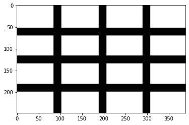
這張圖的大小是 248x389, 然後是灰階圖 (雖然三個 channel,但每個 channel 的值都一樣),type 是 uint8 (0~255)
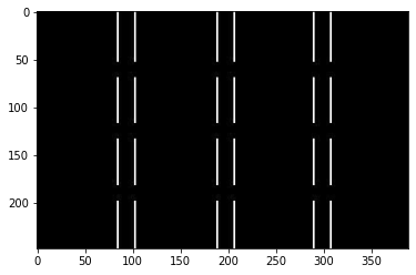
計算 gradient 時,每個像素點,都會算出 x 方向的 gradient 和 y 方向的 gradient.
print(src.min())
print(src.max())

dst = cv2.Sobel(
    src = src,
    ddepth = cv2.CV_16S, # 可選 cv2.CV16S, cv2.CV32
    dx = 1, # 計算 x 軸的一階導數
    dy = 0 # y 軸不計算一階導數
)
print(dst.min())
print(dst.max())

dst2 = cv2.convertScaleAbs(dst)
print(dst2.min())
print(dst2.max())
0
255
-1012
1017
0
255
plt.imshow(dst2);
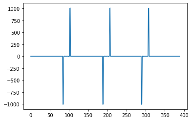
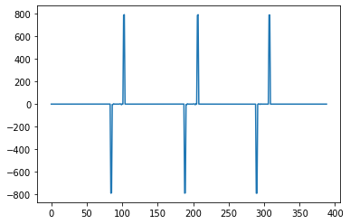
此時如果要看由左到右的 profile,看第一個 row
plt.plot(dst[0,:,0]);
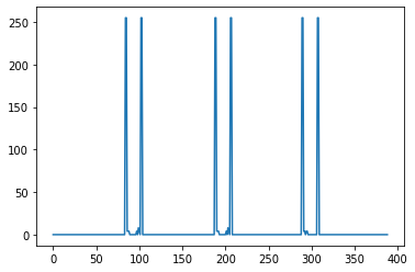
看每個 row 的平均:
plt.plot(dst[:,:,0].mean(axis = 0));
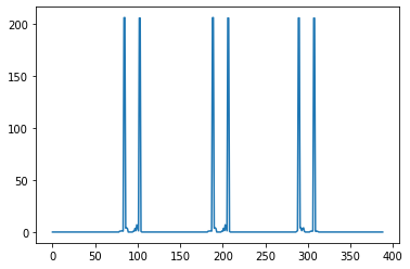
plt.plot(dst2[0,:,0]);
plt.plot(dst2[:,:,0].mean(axis = 0));
# y 方向的
dst = cv2.Sobel(src, cv2.CV_32F, 0, 1)  # 計算 y 軸影像梯度
dst = cv2.convertScaleAbs(dst)          # 將負值轉正值
plt.imshow(dst);

# 完整範例:
dstx = cv2.Sobel(src, cv2.CV_32F, 1, 0)         # 計算 x 軸影像梯度
dsty = cv2.Sobel(src, cv2.CV_32F, 0, 1)         # 計算 y 軸影像梯度
dstx = cv2.convertScaleAbs(dstx)                # 將負值轉正值
dsty = cv2.convertScaleAbs(dsty)                # 將負值轉正值
dst =  cv2.addWeighted(dstx, 0.5,dsty, 0.5, 0)  # 影像融合
plt.imshow(dst);

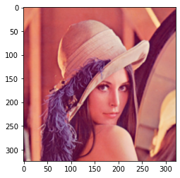
# 應用到實際影像
src = cv2.imread("lena.jpg")
dstx = cv2.Sobel(src, cv2.CV_32F, 1, 0)         # 計算 x 軸影像梯度
dsty = cv2.Sobel(src, cv2.CV_32F, 0, 1)         # 計算 y 軸影像梯度
dstx = cv2.convertScaleAbs(dstx)                # 將負值轉正值
dsty = cv2.convertScaleAbs(dsty)                # 將負值轉正值
dst =  cv2.addWeighted(dstx, 0.5,dsty, 0.5, 0)  # 影像融合

# 將影像從 BGR 轉回 RGB
src = cv2.cvtColor(src, cv2.COLOR_BGR2RGB)
dstx = cv2.cvtColor(dstx, cv2.COLOR_BGR2RGB)
dsty = cv2.cvtColor(dsty, cv2.COLOR_BGR2RGB)
dst = cv2.cvtColor(dst, cv2.COLOR_BGR2RGB)
plt.imshow(src);
plt.imshow(dstx);
plt.imshow(dsty);
plt.imshow(dst);
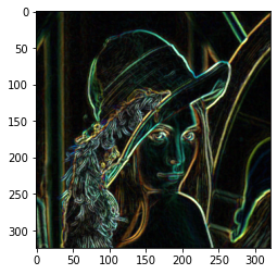
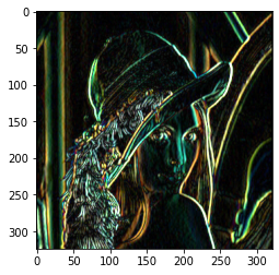
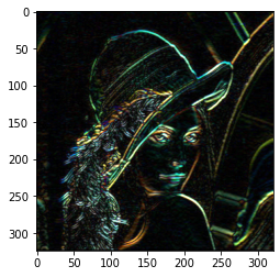
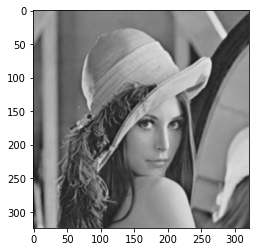
3.3. Scharr
def myplot(img):
    img = cv2.cvtColor(img, cv2.COLOR_BGR2RGB)
    plt.imshow(img);
# Sobel()函數
src = cv2.imread("lena.jpg",cv2.IMREAD_GRAYSCALE) # 黑白讀取
dstx = cv2.Sobel(src, cv2.CV_32F, 1, 0) # 計算 x 軸影像梯度
dsty = cv2.Sobel(src, cv2.CV_32F, 0, 1) # 計算 y 軸影像梯度
dstx = cv2.convertScaleAbs(dstx) # 將負值轉正值
dsty = cv2.convertScaleAbs(dsty) # 將負值轉正值
dst_sobel = cv2.addWeighted(dstx, 0.5,dsty, 0.5, 0) # 影像融合
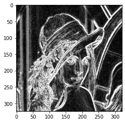
# Scharr()函數
dstx = cv2.Scharr(src, cv2.CV_32F, 1, 0) # 計算 x 軸影像梯度
dsty = cv2.Scharr(src, cv2.CV_32F, 0, 1) # 計算 y 軸影像梯度
dstx = cv2.convertScaleAbs(dstx) # 將負值轉正值
dsty = cv2.convertScaleAbs(dsty) # 將負值轉正值
dst_scharr = cv2.addWeighted(dstx, 0.5,dsty, 0.5, 0) # 影像融合
myplot(src)
myplot(dst_sobel)
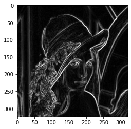
myplot(dst_scharr)
3.4. Laplacian
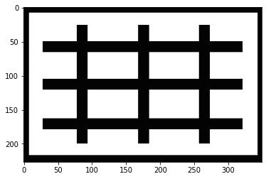
src = cv2.imread("laplacian.jpg")
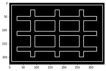
dst_tmp = cv2.Laplacian(src, cv2.CV_32F) # Laplacian邊緣影像
dst = cv2.convertScaleAbs(dst_tmp) # 轉換為正值
print(dst_tmp.max())
print(dst_tmp.min())

print(dst.max())
print(dst.min())
416.0
-482.0
255
0
myplot(src)
myplot(dst)
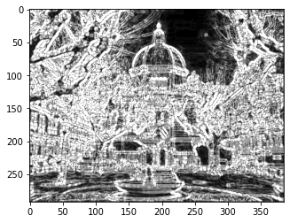
src = cv2.imread("geneva.jpg",cv2.IMREAD_GRAYSCALE)   # 黑白讀取
src = cv2.GaussianBlur(src,(3,3),0)             # 降低噪音
# Sobel()函數
dstx = cv2.Sobel(src, cv2.CV_32F, 1, 0)         # 計算 x 軸影像梯度
dsty = cv2.Sobel(src, cv2.CV_32F, 0, 1)         # 計算 y 軸影像梯度
dstx = cv2.convertScaleAbs(dstx)                # 將負值轉正值
dsty = cv2.convertScaleAbs(dsty)                # 將負值轉正值
dst_sobel =  cv2.addWeighted(dstx, 0.5,dsty, 0.5, 0)    # 影像融合
# Scharr()函數
dstx = cv2.Scharr(src, cv2.CV_32F, 1, 0)        # 計算 x 軸影像梯度
dsty = cv2.Scharr(src, cv2.CV_32F, 0, 1)        # 計算 y 軸影像梯度
dstx = cv2.convertScaleAbs(dstx)                # 將負值轉正值
dsty = cv2.convertScaleAbs(dsty)                # 將負值轉正值
dst_scharr =  cv2.addWeighted(dstx, 0.5,dsty, 0.5, 0)   # 影像融合
# Laplacian()函數
dst_tmp = cv2.Laplacian(src, cv2.CV_32F,ksize=3)    # Laplacian邊緣影像
dst_lap = cv2.convertScaleAbs(dst_tmp)          # 將負值轉正值
myplot(src)

myplot(dst_sobel)
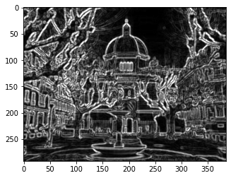
myplot(dst_scharr)

myplot(dst_lap)

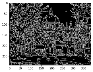
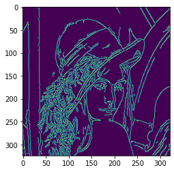
3.5. Canny
src = cv2.imread("lena.jpg",cv2.IMREAD_GRAYSCALE)
dst1 = cv2.Canny(src, 50, 100) # minVal=50, maxVal=100
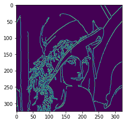
dst2 = cv2.Canny(src, 50, 200) # minVal=50, maxVal=200
plt.imshow(dst1);
plt.imshow(dst2);
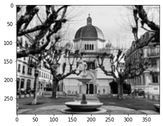
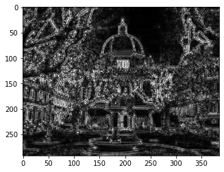
src = cv2.imread("geneva.jpg",cv2.IMREAD_GRAYSCALE)   # 黑白讀取
src = cv2.GaussianBlur(src,(3,3),0)             # 降低噪音
# Sobel()函數
dstx = cv2.Sobel(src, cv2.CV_32F, 1, 0)         # 計算 x 軸影像梯度
dsty = cv2.Sobel(src, cv2.CV_32F, 0, 1)         # 計算 y 軸影像梯度
dstx = cv2.convertScaleAbs(dstx)                # 將負值轉正值
dsty = cv2.convertScaleAbs(dsty)                # 將負值轉正值
dst_sobel =  cv2.addWeighted(dstx, 0.5,dsty, 0.5, 0)    # 影像融合
# Scharr()函數
dstx = cv2.Scharr(src, cv2.CV_32F, 1, 0)        # 計算 x 軸影像梯度
dsty = cv2.Scharr(src, cv2.CV_32F, 0, 1)        # 計算 y 軸影像梯度
dstx = cv2.convertScaleAbs(dstx)                # 將負值轉正值
dsty = cv2.convertScaleAbs(dsty)                # 將負值轉正值
dst_scharr =  cv2.addWeighted(dstx, 0.5,dsty, 0.5, 0)   # 影像融合
# Laplacian()函數
dst_tmp = cv2.Laplacian(src, cv2.CV_32F,ksize=3)    # Laplacian邊緣影像
dst_lap = cv2.convertScaleAbs(dst_tmp)          # 將負值轉正值
# Canny()函數
dst_canny = cv2.Canny(src, 50, 100)             # minVal=50, maxVal=100
plt.imshow(src, cmap = "gray");
plt.imshow(dst_sobel, cmap = "gray");

plt.imshow(dst_scharr, cmap = "gray")
<matplotlib.image.AxesImage at 0x121c81ee0>
plt.imshow(dst_lap, cmap = "gray");
plt.imshow(dst_canny, cmap = "gray");